
ANSYS
Hold Ctrl and scroll to fit to your screen's resolution.

LAMINAR FLOW ANALYSIS OF A 3-D DUCT
Air enters through the small opening of the duct at a rate of 100 in/s and exits out the outlet side. The outlet has a constant static pressure of 0 Pa. For internal flow, the transition to turbulence occurs within a Reynold's number ranging 2000 - 3000. Therefore, the CFD solution of air in the duct is Re = 6106.4, and the flow is turbulent. The flow simulation is conducted to determine the maximum velocity of the air as it exits the duct.

FLOW ANALYSIS IN BALL VALVE WITH Y-CONNECTOR
Air enters through the small opening of the duct at a rate of 100 in/s and exits out the outlet side. The outlet has a constant static pressure of 0 Pa. For internal flow, the transition to turbulence occurs within a Reynold's number ranging 2000 - 3000. Therefore, the CFD solution of air in the duct is Re = 6106.4, and the flow is turbulent. The flow simulation is conducted to determine the maximum velocity of the air as it exits the duct.
STRUCTURAL ANALYSIS OF BIKE FRAME
Air enters through the small opening of the duct at a rate of 100 in/s and exits out the outlet side. The outlet has a constant static pressure of 0 Pa. For internal flow, the transition to turbulence occurs within a Reynold's number ranging 2000 - 3000. Therefore, the CFD solution of air in the duct is Re = 6106.4, and the flow is turbulent. The flow simulation is conducted to determine the maximum velocity of the air as it exits the duct.


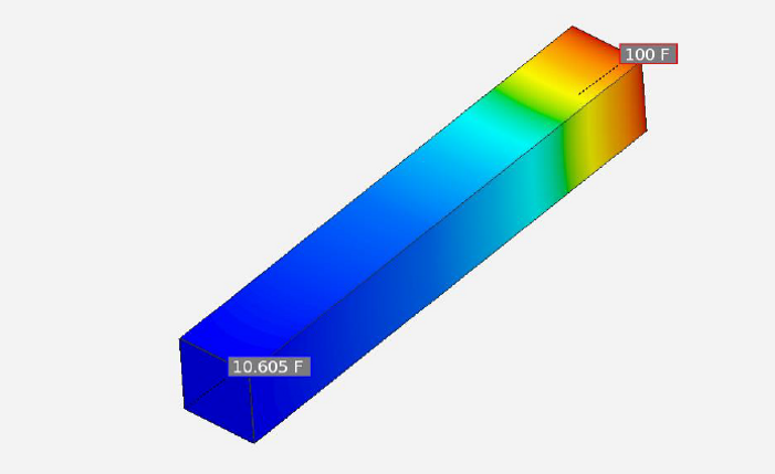
THERMAL ANALYSIS OF STEEL COOLING SPINE
A steel cooling spine of cross-sectional 1.2” x 1.2” and length L = 8” extend from a wall maintained at temperature of 100 F. The thermal conductivity is 6.9034e-3 BTU/s.ft.F. The surface convection coefficient between the spine and the surrounding air is 2.778e-4 BTU/s.ft2.F, the air temperature is 0 F and the tip of the spine is insulated. Thermal analysis is performed to find the temperature at the tip.

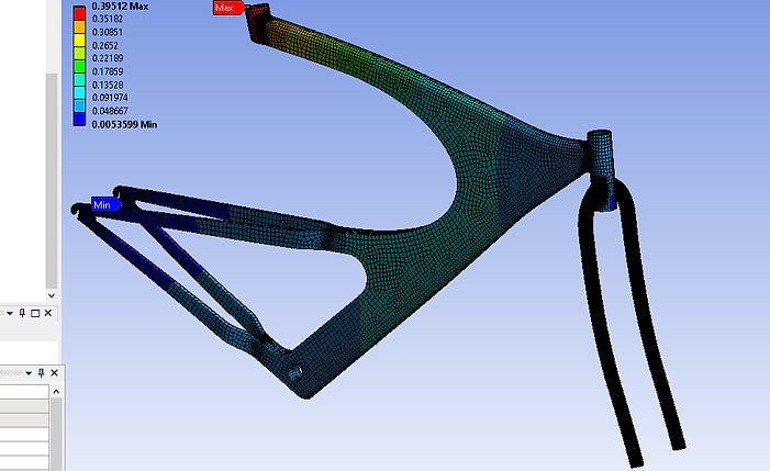
FATIGUE ANALYSIS OF RIDE-ON SUSPENSION
The simplified model of a ride-on suspension made of structural steel is shown here, usually seen in playgrounds. The weight of the ride is 10 lbs. A child weighing 50 pounds stands evenly on the foot holder. The bottom flat face of the suspension is fixed. Fatigue analysis is performed to find the displacement, von-Mises stress and factor of safety as consequence of fatigue damage.

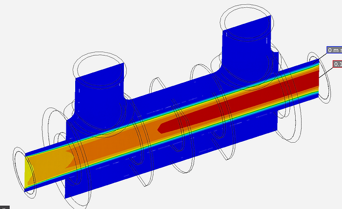
CONJUGATE HEAT TRANSFER ANALYSIS OF CROSS FLOW HEAT EXCHANGER
The steel heat exchanger is subjected to the cross-flow of air and water at different temperatures. Due to fluid flow, the heat exchanger is also subjected to the fluid temperature. Heat Transfer analysis is performed to find the thermal efficiency and the factor of safety of the heat exchanger.
Laminar Flow Analysis of 3-D Duct
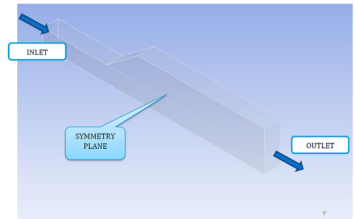
Geometric Model of Duct
This simulation is performed using ANSYS Workbench. Initially, the duct is cut extruded from the center XY-plane and the fluid domain is set by selecting and "filling" the inner walls of the remaining side of the duct. The original body of the duct is suppressed. Next, the regions for inlet, outlet and symmetric plane are set. Lastly, a fine mesh with inflation of 10 layers is scoped on the entire body.
In CFX simulation, the fluid is defined to be air at 25 C and turbulence is set to laminar. The boundary conditions are set as 100 in/s at inlet, symmetry plane as symmetric, and 0 Pa for average static pressure at outlet. The default domain is set to No Slip Wall. Finally, the CFX simulation solver is run to achieve the results below.
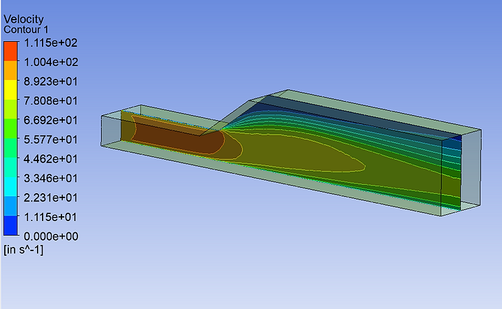
Velocity Contour Plot on Symmetric Plane
In this contour plot, the velocity is maximum at the inlet, where its near to 100 in/s. As the air travels across the bend of the duct where it expands in width, the velocity of the air decreases to an average of 72 in/s around the center and much lower to 14 in/s around the top surface. This is due to laminar flow and the air moves in a direction parallel to the duct as it enters.
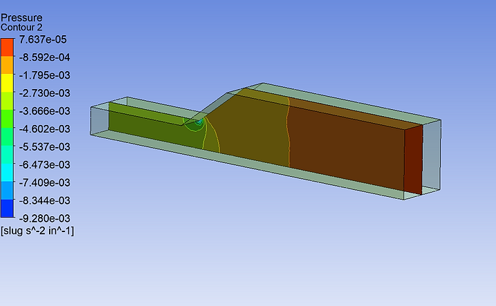
Pressure Contour Plot on Symmetric Plane
This contour plot shows the pressure distribution across the duct. It can be observed that the pressure is very low around the inlet region, since the air enters at constant pressure in a laminar flow. The pressure gradually increases to a maximum of 0.0439 Pa at the outlet region, which is still very low.

Velocity Contour Plot at Outlet
This velocity contour plot at the outlet of the duct shows that air exits the duct at a faster rate through the area that is straight from the inlet. The velocity of air exiting from the region near the top surface is almost negligible, compared to that in the bottom surface parallel to the inlet. This proves that air in laminar flow will most likely stay in laminar flow unless it passes through an obstacle.
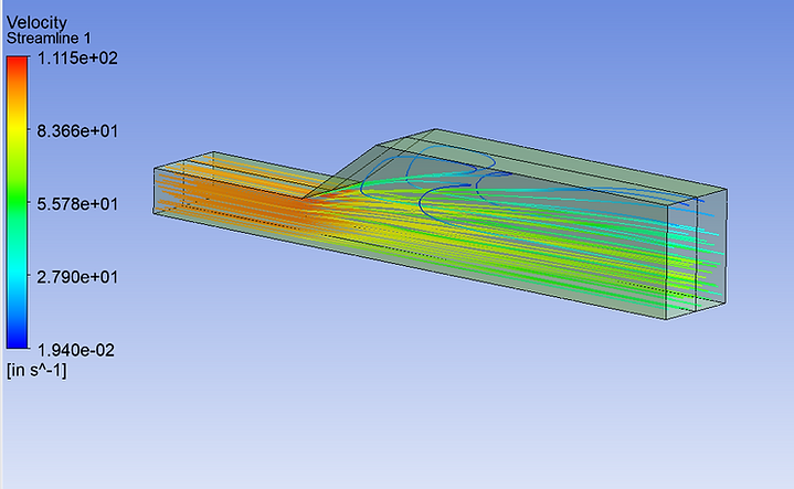
Streamline Plot Across Duct
This streamline plot of air flowing through the duct further reinforces the statement that air in laminar flow will stay in laminar flow unless it faces an obstacle. Very little air suffers from turbulence near the bend but most of it flows straight through the duct and exits from the bottom region of the outlet.
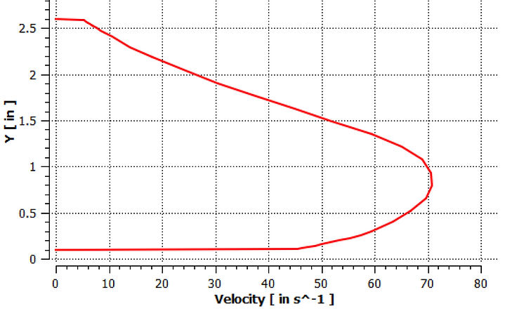
Velocity Profile at Outlet
From the velocity profile generated, it can be concluded that the flow is fully developed at the outlet, with a maximum velocity of 71 in/s.
Flow Analysis in Ball Valve with Y-Connector
Landing Gear Assembly
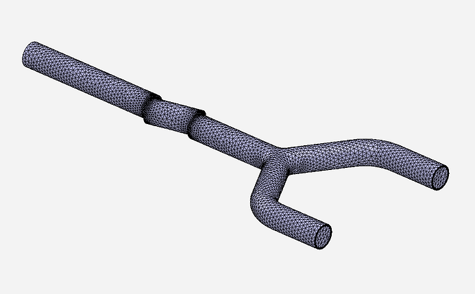
Geometric Model of Pipe with Ball Valve
The model is designed on SolidWorks as an assembly of the inlet pipe, ball valve and the Y-connector pipes. The .STEP file is imported into ANSYS AIM Discovery. It is meshed (refined near the ball valve edges) and the fluid domain is set by putting lids on the pipe openings. The fluid is defined to be to water at 25 C. The entire body is set as a no slip wall.
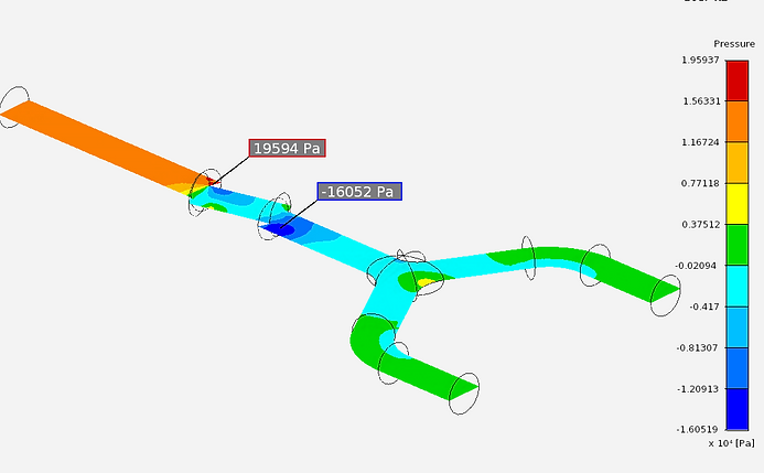
Pressure Contour Plot on Symmetric Plane
This pressure contour plot shows that the maximum pressure is at the region where water enters the ball valve (19594 Pa) and the minimum is where the water exits the valve (-16052 Pa). This is because the ball valve is half open and water pressure builds up at the inlet pipe but the mass flow rate is reduced as it flows to each outlet. The pressure increases slightly at each outlet of the Y-connector.

Velocity Contour Plot on Symmetric Plane
The velocity contour plot shows that water enters at about 4 m/s but increases at the ball valve as the pressure builds up. The maximum velocity is 7.7882 m/s, where the water exits the ball valve. It then slows down to a very low flow rate as it flows out through each of the outlets of the Y-connector.

Velocity Streamline Plot on Symmetric Plane
The velocity streamline plot shows that water enters the pipe in laminar flow. Upon entering the ball valve, the velocity increases suddenly to a maximum of 7.9174 m/s and then gradually decreases as it flows out of each outlet pipes of the Y-connector. The streamline demonstrates slight turbulence near the split bend of the Y-connector.

Streamline Plot Through Ball Valve
This time distribution streamline plot shows that water enters the pipe at a faster rate compared to exiting through the outlets. Overall, it takes about 0.15 seconds for water to flow through the entire pipe at a mass flow rate of 0.5 kg/s.
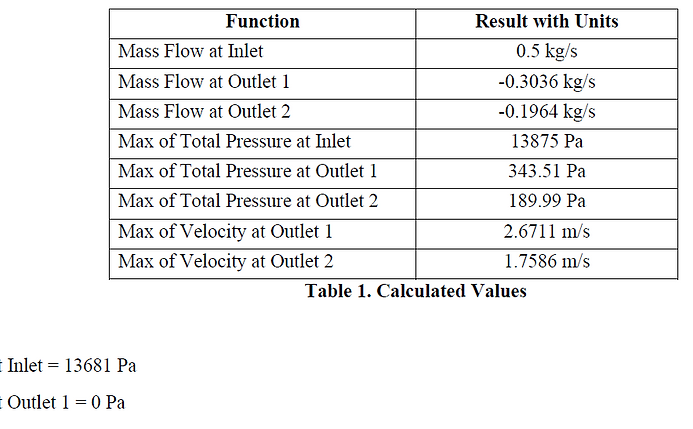
Calculated Values
The table on the left show the calculated values of mass flow rate, maximum total pressure and maximum velocity at each boundary, determined from ANSYS AIM.
Structural Analysis of Bike Frame

Geometric Model of Bike Frame
The bike frame is designed on SolidWorks and exported as a .stp file so simulations can be performed on it using ANSYS Workbench. Three loading conditions are prepared, therefore three structural analyses are linked together. The material is defined to be Titanium Alloy. For the first structural analysis, displacement loading condition is set on both the rear wheel axle mount and the x-component is kept free to move. Next, the two end faces of the front fork has another similar displacement. Lastly, the cylindrical face of the hole has a free-to-move y-component displacement.
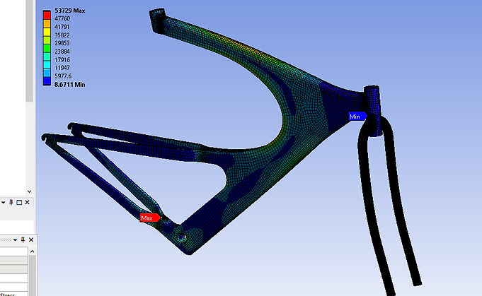
Sitting Load - Stress Contour Plot
For the sitting load constraints, one ramped force of -1424 N is placed on the flat circular surface of the seat mount. This simulates the rider's weight fully acting vertically downwards on the seat mount. The equivalent stress (von-Mises) plot is generated. It is observed that the maximum stress of 53729 psi occurs near the region where it forks into two bars for the rear wheel axle mounts. The minimum stress of 8.62 psi occurs at the handle-bar mount.
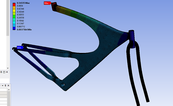
Sitting Load - Deformation Contour Plot
This deformation contour plot shows one load acting on the flat circular surface of the seat mount. The maximum deformation of 0.54 inch occurs near the seat mount and proportionately decreases across the upper beam.

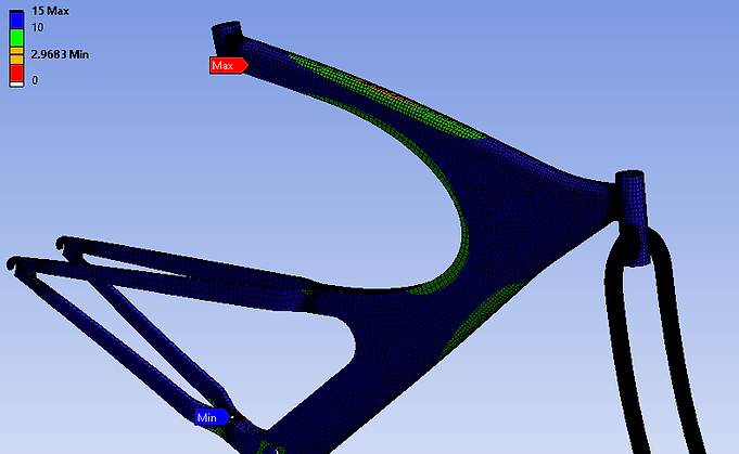
Sitting Load - Safety Factor Plot
The factor of safety plot shows that the bike frame will not fail under the static load of -1454 N. The minimum factor of safety occurs near the upper beam connecting the seat mount and handlebar mount. the maximum factor of safety is 15, which is throughout the bike frame.
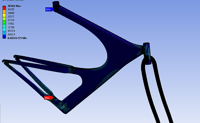
Standing Load - Stress Contour Plot
The standing load of -1545 N acting on the inner face of the pedal hole generates the stress contour plot shown here. It can be observed that the stress distribution is very minimal, acting mostly in the axle region and handlebar mount. The maximum stress is 38.37 psi, acting at the fork of the pedal hole. The minimum stress of 0 psi occurs directly below the seat.

Standing Load - Deformation Contour Plot
The deformation plot shows a maximum deformation of 0.19 inch occurring at the fork where the front axle is located. There is some amount of deformation throughout the bike frame under the standing load of -1454 N, mostly around 0.086 inches.

Standing Load - Safety Factor Plot
This safety factor plot shows that the bike frame will not fail under the standing load of -1545 N acting on the inner faces of the pedal hole.

Combo Loads
Next, a combination of loads is placed on the faces shown here. A sitting load of 224.09 lb acts on the upper face of the seat mount, a standing load of 48.019 lb acts on the inner face of the pedal hole, and a force of 48.019 lb acts on the handlebar mount. These forces represent the distribution of an average person's weight on a bike.
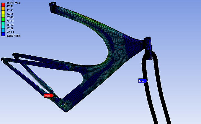
Combo Loads - Stress Contour Plot
The combo loads generate a maximum stress of 45442 psi acting near the fork near the pedal hole. The minimum stress is 4.68 psi. An average stress of 15150 psi acts along the main body of the frame and increases slightly to 22000 psi at the bar between seat mount and handlebar mount.

Combo Loads - Deformation Contour Plot
Next, a combination of loads is placed on the faces shown here. A sitting load of 224.09 lb acts on the upper face of the seat mount, a standing load of 48.019 lb acts on the inner face of the pedal hole, and a force of 48.019 lb acts on the handlebar mount.
Combo Loads - Safety Factor Plot
The bike frame will not fail under the combo loads. The safety factor is relatively lower near the arm connecting the seat mount and handlebar mount compared to the rest of the body. However, it is still too high for the frame to fracture under these loads.
Explicit Dynamic Analysis of Bullet Casing
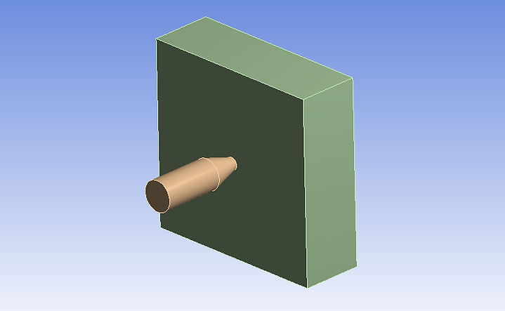
Geometric Model of Bullet and Wall
The copper alloy bullet casing is modeled to strike the fixed steel wall at a high impact velocity of 400 m/s for 0.0005 seconds. The bullet casing has a maximum equivalent plastic strain EPS of 0.75 and a thickness of 1 mm. To simulate the fragmentation, it is assumed that the copper will be torn apart when the plastic strain is larger than 75%.

Deformation at 2.5009E-05 secs
The bullet casing strikes the wall at 400 m/s (faster than speed of sound) and begins to deform. At 2.5009E-05 seconds, the tip of the bullet shatters.

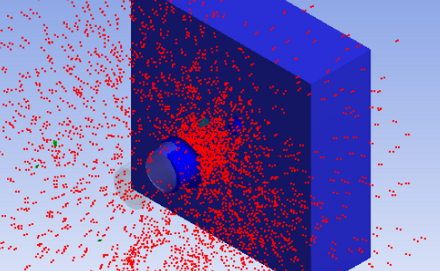
Deformation at 2.5E-04 secs
At 2.5E-04 seconds, the majority of the casing shaft explodes into particles that spread uniformly and concentrically. A larger portion of the shaft is also displaced along with the particles.
Deformation at 5E-04 secs
At 5E-04 seconds, the bullet casing is almost fully shattered into particles that travel concentrically in all directions.
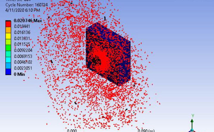
Final Solution
The final solution is shown here, with the bullet casing completely fragmented upon high impact with the steel wall. The equivalent elastic strain is found to be 0.0207 m/m.

Effective Strain
The effective strain (geometric strain), derived as the ratio of yield strength (2.8E+08 Pa)and the tangent modulus (1.15E+09 Pa)of the bullet casing, is found to be a maximum of 1.0072.
Buckling of a Circular Arch
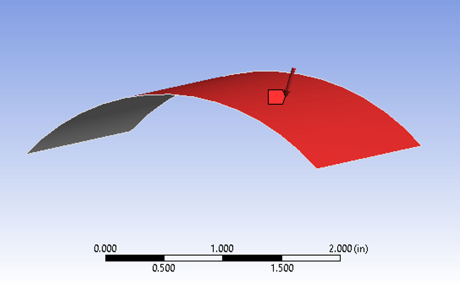
Geometric Model of Circular Arch
The arch has a cross-section of 5 mm x 50 mm and a mean radius of 50 mm. The arch is made of steel and subjected to a load of 1 MPa. Both the straight edges are simply supported. The objective is to find the buckling load factor (Load Multiplier) for 4 buckling modes and the maximum normal stress in the x-direction of the cylindrical surfaces of the hole. The material is set to buckling steel, with Young's Modulus of 20000 MPa and Poisson's ratio of 0, to compare to theoretical solution. The thickness of the arch is 5 mm.
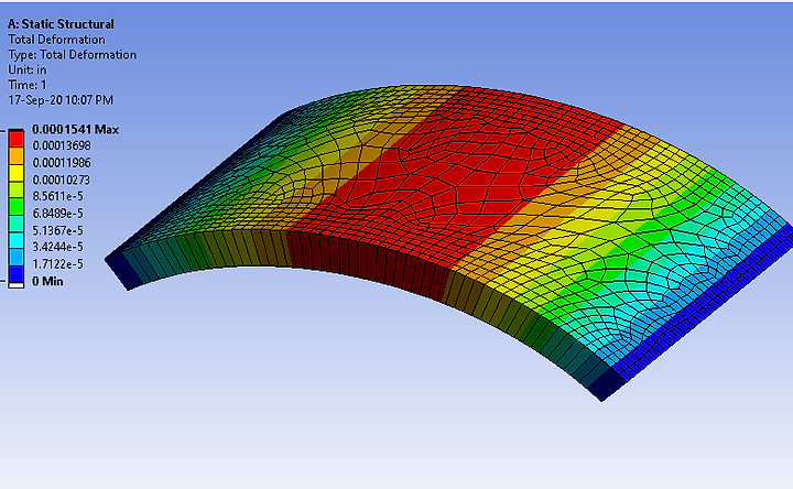
Total Deformation Banded Plot
The total deformation is shown in banded curves across the circular arch when subjected to 1 MPa of uniform pressure. The maximum deformation of 1.541E-4 inches occurs in the center region. The average deformation is calculated to be 8.504E-05 inches.
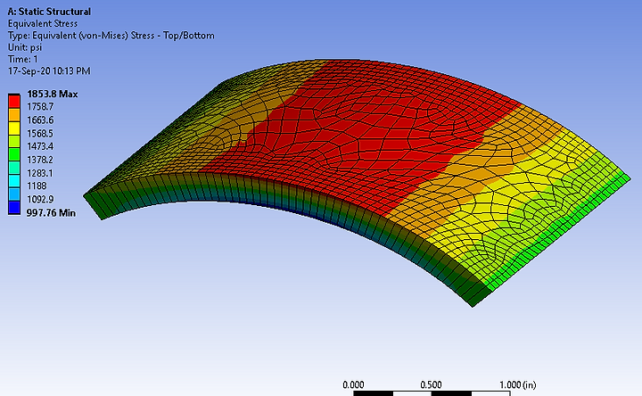
Equivalent Stress Banded Plot
The equivalent (von-Mises) stress plot is shown here. The maximum von-Mises stress of 1853.8 psi occurs along the center region where the bend occurs. The minimum stress is 997.76 psi that occurs along the inner surface of the arch. The average stress is calculated to be 1429.7 psi.

Eigenvalue Buckling: Mode 1
In Mode 1, the load multiplier is 246.36, with a maximum total deformation of 0.05 inches.
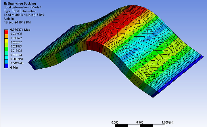
Eigenvalue Buckling: Mode 2
In Mode 2, the load multiplier is 550.9, with a maximum total deformation of 0.039 inches.
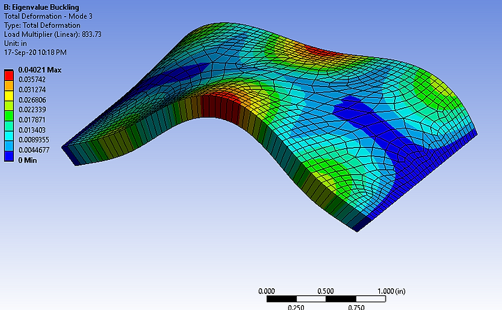
Eigenvalue Buckling: Mode 3
In Mode 3, the load multiplier is 833.73, with a maximum total deformation of 0.04 inches.
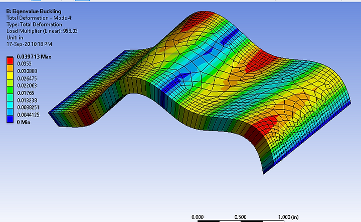
Eigenvalue Buckling: Mode 4
In Mode 4, the load multiplier is 958.03, with a maximum total deformation of 0.04 inches. This is almost the same as Mode 3.
Thermal Analysis in Steel Cooling Spine
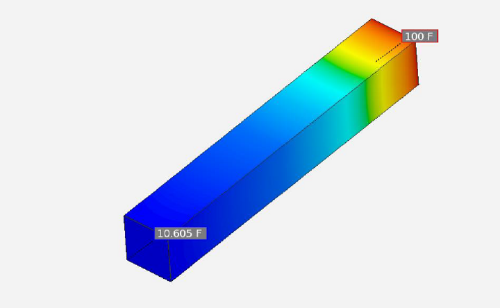
Temperature Contour Plot
The temperature contour plot generated from running the thermal analysis with the given parameters shows that the temperature at the tip is 10.605 F. Therefore, the cooling spine is functional in its purpose.
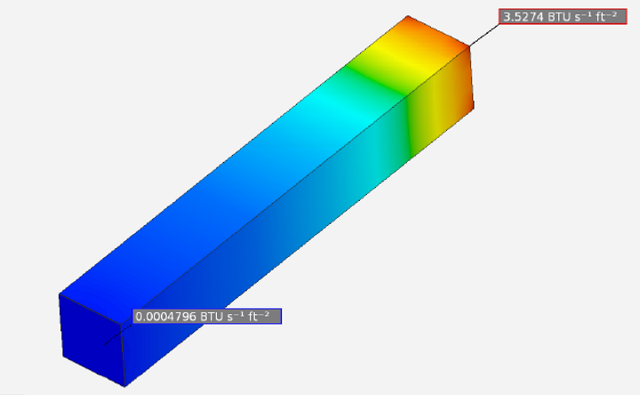
Heat Flux Contour Plot
The heat flux contour plot shows that heat is slowly dissipating into the ambient surrounding air along the length of the spine. The heat flux at the tip is negligible, since it is insulated. The maximum heat flux of 3.5274 BTU/s.ft^2 occurs near the wall.
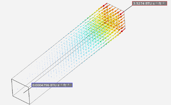
Heat Flux Vector Plot
The heat flux vector plot shows the direction that the heat is dissipating along the cooling spine.
Fatigue Analysis of Ride-On Suspension

Temperature Contour Plot
The simplified model of a ride-on suspension made of structural steel is shown here, usually seen in playgrounds. The weight of the ride is 10 lbs. A child weighing 50 pounds stands evenly on the foot holder. The bottom flat face of the suspension is fixed. Fatigue analysis is performed to find the criterion below.
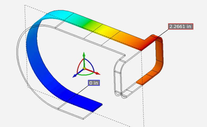
Displacement Contour Plot
The displacement contour plot shows the maximum displacement of 2.2661 inches occurs in the upper part of the foot holder, where it connects to the suspension.
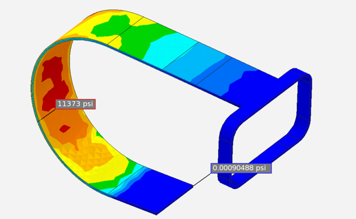
von-Mises Stress Contour Plot
The equivalent von-Mises contour plot shows the maximum stress of 11373 psi occurs near the bend of the suspension between the arm holding the foot-holder and the fixed bottom.

Safety Factor Plot
The factor of safety plot shows that the ride-on suspension will not fail under the applied loads. This is because the minimum factor of safety is still above 1, along the main bend of the suspension.
Spur Gear Tooth Strength Analysis
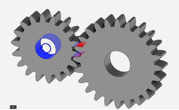
Geometric Model of Gear Train
A 18-tooth pinion gear with a diametral pitch of 6 meshes with a 24-tooth gear. The face width of both the gears is 0.75 inches. Strength analysis is performed to check if the gear train is safe during transmission of torque of 6000 lb-in. The interface conditions are set as frictionless contact between the mating gear teeth.

Displacement Banded Plot
The displacement banded plot shows how the 18-tooth pinion gear displaces when the 20-tooth one is axially supported. The maximum displacement of 0.00380 inches on the tip of the teeth.

von-Mises Stress Contour Plot
The von-Mises contour plot shows that the maximum stress occurs in the regions where the gear teeth of both gears are in contact with each other. The maximum von-Mises stress is 3.988E05 psi, which is enormous. However, since the stress acts in such a small area, it is bearable.
Conjugate Heat Transfer Analysis of Cross-Flow Heat Exchanger

Geometric Model
Air at a temperature of 327 C flows through the center tube from the near inlet end at 0.1 m/s and exits at 0 Pa static pressure from the farther outlet end. Water at a temperature of 20 C circulates around the center tube at a mass flow rate of 0.02 kg/s from the upper inlet to upper outlet at 0 Pa static pressure. The heat transfer coefficient is 5 W/m^2.C and convection temperature is 15 C. The inlet and outlet pipes are insulated.
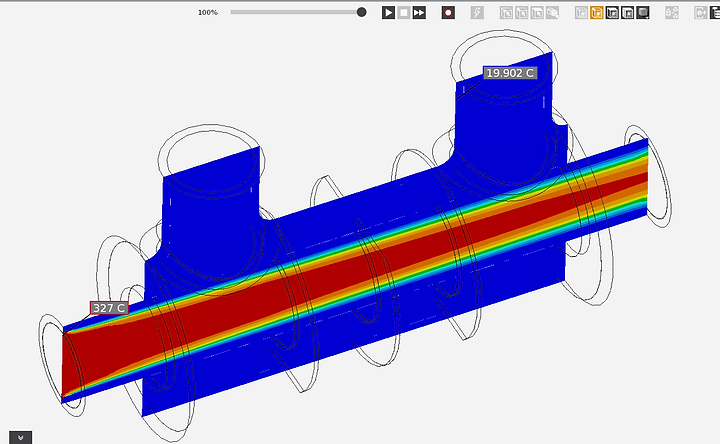
Temperature Contour Plot
The temperature contour plot shows that the temperature of the air flow decreases as it flows from inlet to the outlet. The water at the inlet is at a minimum temperature of 19.902 C.
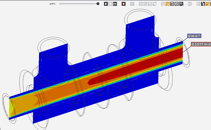
Velocity Contour Plot
The velocity contour plot shows that the velocity of the air increases as it flows to the outlet. The maximum velocity of 0.1577 m/s is at the outlet. This is because the outlet pressure is 0 Pa and the air is forced to accelerate towards the low pressure region.
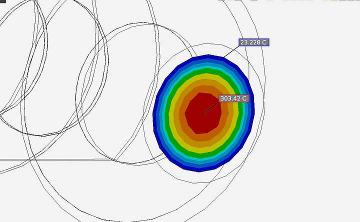
Temperature Contour Plot at Outlet
The temperature contour plot at the outlet shows concentric bands of temperature that decreases from the center to the cylindrical surface of the outlet pipe. The maximum temperature of air is 303.42 C and the minimum is 23.23 C. These temperatures are significantly less than the inlet temperature of 327 C.

Streamline Plot
The streamline plot shows the linear flow of air through the central pipe and the turbulent flow of water that circulates around the central pipe to cool down the air.

Equivalent Stress Contour Plot
The equivalent stress contour plot shows that the maximum equivalent stress of 7.55E07 Pa occurs at the cylindrical surface of the inlet pipe for air.
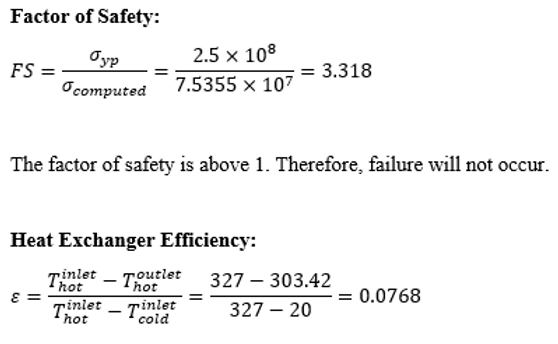
Calculations
The factor of safety is calculated to be 3.318, which proves that the heat exchanger will not fracture under the stress caused by the air flow. The heat exchanger efficiency is calculated to be 7.68%, which is moderately efficiency for a simple heat exchanger. The efficiency is much higher when air inlet velocity is lower. The efficiency increases by 5.38% as air inlet velocity is lowered from 1 m/s to 0.1 m/s.